Introduction: The Need for Survey Weights

Surveys are an essential tool for gathering information and understanding public opinion on various issues. The success of survey-based research largely depends on the sampling procedure used. When sampling units do not have equal probabilities of selection, survey weights become crucial to ensure that statistics derived from the sample accurately represent the target population.

Typically, a survey weight for each unit is calculated as the inverse of its probability of being selected. In a simple random sample, this would be 1/N, where N is the total population size, making the weight uniform across all units. However, more complex survey designs—such as stratified, clustered, or multistage sampling—require different weights since each unit may represent varying numbers of people from the target population.

Even with accurately calculated initial weights, the sample might not perfectly reflect the population due to the inherent randomness of sampling, or factors like non-response or coverage biases. To address these discrepancies, sample weights can be adjusted to better align with known population totals. This process, known as sample balancing, will be further explored with a focus on a specific technique called ‘raking’ in the next section.

An Overview of the Raking Methodology for Survey Weights

Raking, also known as iterative proportional fitting, is a post stratification procedure that can be used to adjust survey weights to better align with known population totals. It is most commonly used to account for non-response and non-coverage biases, but can account for a range of biases in the design and implementation of a survey. Raking enhances the representativeness and accuracy of survey results, assuming accurate population totals.

Here are some commonly recommended ‘best practices’ for raking:

Base weights:

Starting with base weights, initial weights based on the inverse probability of selection, is a standard approach (Battaglia et al., 2009).

Variable selection:

Choosing relevant variables is critical. Typically, these include demographic information and key survey topics. For instance, political affiliation might be used for a survey on public policy opinions (Pew Research Center, 2018).

Collapse small cells:

It is recommended to merge smaller categories that represent less than 2% of the sample or control totals to prevent issues with convergence and prevent overfitting (Battaglia et al., 2009)(Oh and Scheuren, 1978).

Weight trimming:

Limiting the number of iterations and trimming outlier weights helps prevent overfitting. Weights significantly larger than average (e.g. 5x) should be truncated to maintain balance (Battaglia et al., 2004)

Model evaluation:

Often, demographic discrepancies exceeding 5 percentage points are “notable” and discrepancies less than 2 percentage points are not. Discrepancies in the 2 to 5 point range may be notable if the characteristic is of special interest for the study or is strongly associated with key outcome variables (Debell & Krosnick, 2009)
It’s best to examine the effects of raking on variables not used as raking factors. If these estimates show a greater difference from the benchmarks using the new weights, consider raking with a revised poststratification approach (Debell & Krosnick, 2009)

The following section will outline the raking algorithm and walk through a simple demonstration of how the raking process can be used to improve alignment with known population values.

Simple Raking Example

This section provides a high level description of the raking algorithm and then walks through a simple example using two binary variables to illustrate the raking process.

Raking steps:

Take each row in turn and multiply each entry in the row by the ratio of the population total to the weighted sample total for that category
- The row totals of the adjusted data should agree with the population totals for that variable. The weighted column totals of the adjusted data, however, may not yet agree with the population totals for the column variable.
Take each column and multiply each entry in the column by the ratio of the population total to the current total for that category.
- Now the weighted column totals of the adjusted data agree with the population totals for that variable, but the new weighted row totals may no longer match the corresponding population totals.
Continue alternating between the rows and the columns.
- Close agreement on both rows and columns is usually achieved after a small number of iterations.
The result is a tabulation for the population that reflects the relation of the two control variables in the sample.
Raking can also adjust a set of data to control totals on three or more variables. In such situations the control totals often involve single variables, but they may involve two or more variables.

Simple Raking Example

	Child	Adult	Row Total
Urban	30	20	50
Rural	20	30	50
Column Total	50	50	100

Desired population totals:

Urban: 60, Rural: 40
Child: 40, Adult: 60

Adjusting the rows first to match the locality population totals:

Urban adjustment ratio: 60 / 50 = 1.2
Rural adjustment ratio: 40 / 50 = 0.8

Adjusted rows:

	Child	Adult	Row Total
Urban	36	24	60
Rural	16	24	40
Column Total	52	48	100

Now, the row totals match the population totals for locality. However, the column totals for age groups are still off.

Adjusting columns to match the age group population totals:

Child adjustment ratio: 40 / 52 ≈ 0.7692
Adult adjustment ratio: 60 / 48 = 1.25

Adjusted columns:

	Child	Adult	Row Total
Urban	27.69	30	57.69
Rural	12.31	30	42.31
Column Total	40	60	100

Readjusting the rows to match the locality population totals:

Urban adjustment ratio: 60 / 57.69 = 1.04
Rural adjustment ratio: 40 / 42.31 = 0.945

Adjusted rows:

	Child	Adult	Row Total
Urban	28.80	31.20	60
Rural	11.61	28.36	40
Column Total	40.44	59.56	100

Readjusting the columns to match the age population totals:

Child adjustment ratio: 40 / 40.44 = 0.989
Adult adjustment ratio: 60 / 59.56 = 1.007

	Child	Adult	Row Total
Urban	28.49	31.43	59.92
Rural	11.51	28.57	40.08
Column Total	40	60	100

At a certain point, the algorithm determines that the marginal populations are “close enough” to the target population — this is convergence. You are able to specify the convergence criterion when setting up the raking procedure. One simple definition of convergence requires that each marginal total of the raked weights be within a specified tolerance of the corresponding control total. In the rake() function in R, convergence is reached if the maximum change in a table entry is less than epsilon (default = 1).

It is harder to visualize when raking on more variables, but the process is the same. You continue making adjustments until the marginal sample populations are “close enough” to the target.

Case Study: Raking to Improve Representativeness in National Household Survey

Background:

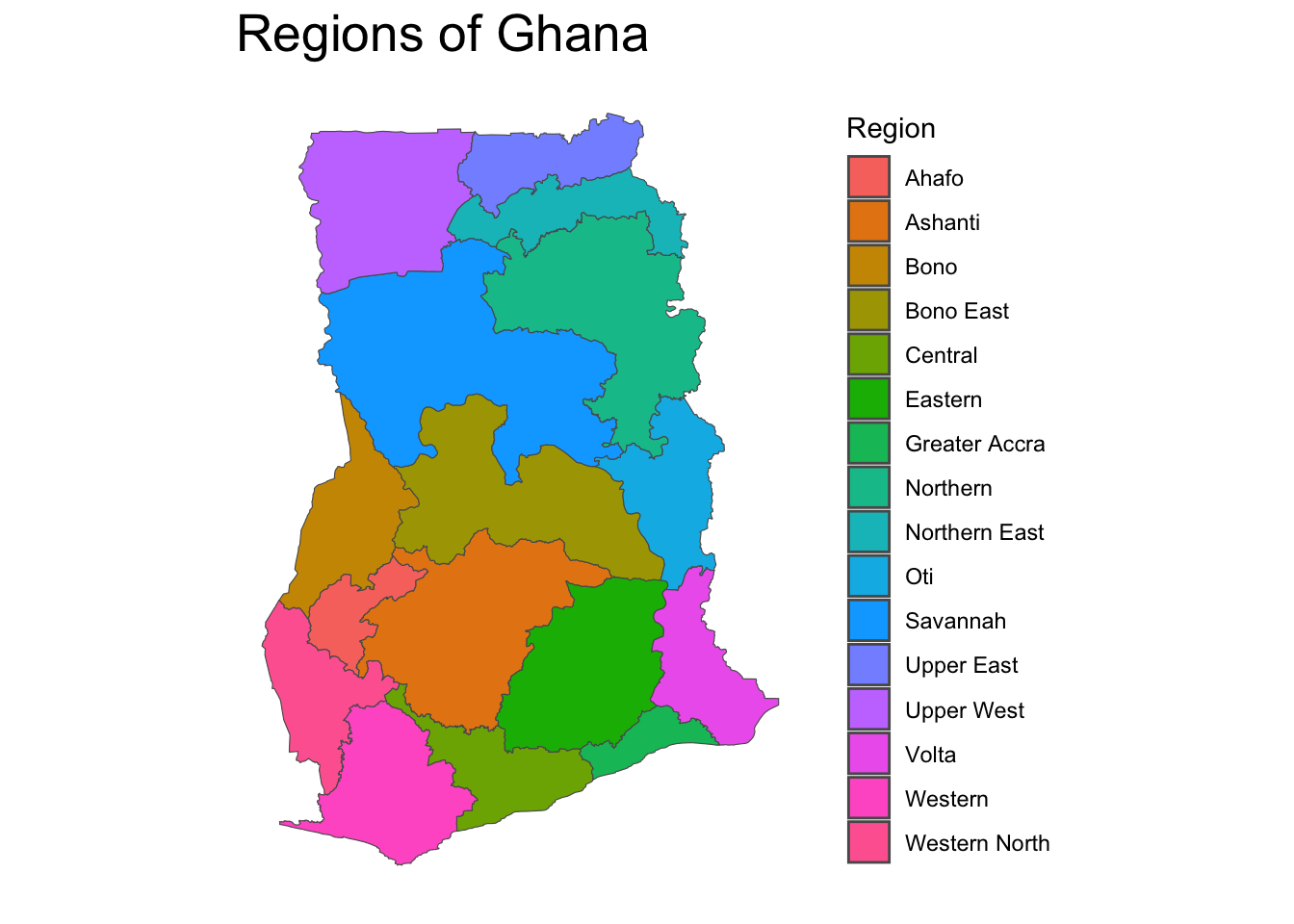
As part of the Combating Household Air Pollution (CHAP) project, we applied raking to a national household survey on fuel use in Ghana. The CHAP project is a collaborative effort from several research institutions: Columbia University, UC Santa Barbara, and the Kintampo Health Research Center in Ghana. For the fuel survey, we also partnered with the Ghana Statistical Service to conduct the sampling and interviews.

The CHAP survey employed a multistage, cluster approach to the sample. A total of 370 enumeration areas (EAs) and 20 households within each EA were sampled for a total sample size of 7,400 households. Ghana’s 16 regions were used for stratification, as well as the classification of an EA as either urban or rural.

Initial survey weights were calculated based on the probability of selecting an EA and a household within it. Discrepancies between our survey results and the census data from the Ghana Statistical Services (GSS) prompted us to employ raking to refine our weights.

Set Up:

We tested various raking models using the survey package in R, starting with base weights and adjusting for different sets of variables. To address issues with small cell sizes, regional data was consolidated into larger groupings. The process and rationale for these adjustments are detailed below.

y* indicates that the measurement is obtained through the regional cross distribution.
Stat	Rake 1	Rake 2	Rake 3	Rake 4
Total urban/rural households	y	y*	y	y*
Total households in each region	y	y*	y	y
Regional urban/rural households		y		y
Total primary fuel source			y	y*
Regional primary fuel source				y

Expand the code blocks below to examine how we set up the raking procedure and complete raking for each of these models.

Setting up the Population Totals for Raking

Code

### urban/rural total
pop.urban_rural_str <-
  data.frame(
    urban_rural_str = c("urban", "rural"),
    Freq = c(
      subset(gss, region == "Total")$hh_pop_urban,
      subset(gss, region == "Total")$hh_pop_rural
    )
  )

### primary fuel categories 

hh_pop_tot <- subset(gss, region == "Total")$hh_pop

frac_lpg <- subset(gss, region == "Total")$fuel_lpg / subset(gss, region == "Total")$hh_pop_fuel

frac_char <- subset(gss, region == "Total")$fuel_char / subset(gss, region == "Total")$hh_pop_fuel

frac_wood <- subset(gss, region == "Total")$fuel_wood / subset(gss, region == "Total")$hh_pop_fuel
  

pop.primary_fuel <-
  data.frame(
    collapsed_fuel = c("none_other", "wood", "LPG", "charcoal"),
    Freq = c(
      round((1 - (frac_lpg + frac_wood + frac_char)) * hh_pop_tot, 0),
      round(frac_wood * hh_pop_tot, 0),
      round(frac_lpg * hh_pop_tot, 0),
      round(frac_char * hh_pop_tot, 0)
    )
  )


### regional 2021 HH populations 
gss_regional <- filter(gss, region != "Total") 

pop.region_hh <- data.frame(
  region = gss_regional$region,
  Freq = gss_regional$hh_pop
)




# regional main fuel 
#specify known main fuel population values for each of the regions 
pop.region_main_fuel <- gss_regional %>% 
  mutate(none_other = fuel_none + fuel_other) %>%
  rename(LPG = fuel_lpg, 
         wood = fuel_wood, 
         charcoal = fuel_char) %>%
  select(region, none_other, wood, LPG, charcoal) %>%
  
  #apply scaling factor so population matches GSS total value
  mutate(none_other = round(none_other * subset(gss, region == "Total")$hh_pop/subset(gss, region == "Total")$hh_pop_fuel, 0),
         LPG = round(LPG * subset(gss, region == "Total")$hh_pop/subset(gss, region == "Total")$hh_pop_fuel,0),
         wood = round(wood * subset(gss, region == "Total")$hh_pop/subset(gss, region == "Total")$hh_pop_fuel, 0),
         charcoal = round(charcoal * subset(gss, region == "Total")$hh_pop/subset(gss, region == "Total")$hh_pop_fuel, 0))

northern <- pop.region_main_fuel %>%
  filter(region %in% c("Upper East", "Upper West", "North East", "Northern", "Savannah", "Oti", "Bono", "Bono East", "Ahafo")) %>%
  summarise(
    region = "northern",
    none_other = sum(none_other),
    wood = sum(wood),
    LPG = sum(LPG),
    charcoal = sum(charcoal)
  )


middle <- pop.region_main_fuel %>%
  filter(region %in% c("Ashanti", "Eastern")) %>%
  summarise(
    region = "middle",
    none_other = sum(none_other),
    wood = sum(wood),
    LPG = sum(LPG),
    charcoal = sum(charcoal)
  )

southeast <- pop.region_main_fuel %>%
  filter(region %in% c("Greater Accra", "Volta")) %>%
  summarise(
    region = "southeast",
    none_other = sum(none_other),
    wood = sum(wood),
    LPG = sum(LPG),
    charcoal = sum(charcoal)
  )

southwest <- pop.region_main_fuel %>%
  filter(region %in% c("Central", "Western", "Western North")) %>%
  summarise(
    region = "southwest",
    none_other = sum(none_other),
    wood = sum(wood),
    LPG = sum(LPG),
    charcoal = sum(charcoal)
  )

collapsed_region_primary_fuel <- bind_rows(northern, middle, southeast, southwest)


#Combine primary fuel with each row specifying which is applicable 
pop_region_primary_fuel_long <- collapsed_region_primary_fuel %>%
  pivot_longer(cols = c(none_other, wood, LPG, charcoal), names_to = "collapsed_fuel", values_to = "Count") #names need to match what is in the survey!!

# reformat this data so each row is a household (necessary for creating pop.table below)
pop_region_primary_fuel_long <- pop_region_primary_fuel_long %>%
  uncount(Count) %>%
  rename(collapsed_region = region)

#create table of LPG main stove by collapsed regions
pop.table_primary_fuel <- xtabs(~collapsed_region+collapsed_fuel, pop_region_primary_fuel_long)




# regional urbanicity 
#regional 2021 HH populations 
pop.region_urban_rural_hh <- gss_regional %>%
  select(region, hh_pop_rural, hh_pop_urban) %>%
  rename(rural = hh_pop_rural, 
         urban = hh_pop_urban)


northern <- pop.region_urban_rural_hh %>%
  filter(region %in% c("Upper East", "Upper West", "North East", "Northern", "Savannah", "Oti", "Bono", "Bono East", "Ahafo")) %>%
  summarise(
    region = "northern",
    urban = sum(urban),
    rural = sum(rural)
  )


middle <- pop.region_urban_rural_hh %>%
  filter(region %in% c("Ashanti", "Eastern")) %>%
  summarise(
    region = "middle",
    urban = sum(urban),
    rural = sum(rural)
  )

southeast <- pop.region_urban_rural_hh %>%
  filter(region %in% c("Greater Accra", "Volta")) %>%
  summarise(
    region = "southeast",
    urban = sum(urban),
    rural = sum(rural)
  )

southwest <- pop.region_urban_rural_hh %>%
  filter(region %in% c("Central", "Western", "Western North")) %>%
  summarise(
    region = "southwest",
    urban = sum(urban),
    rural = sum(rural)
  )

collapsed_region_urban_rural_hh <- bind_rows(northern, middle, southeast, southwest)


#Combine LPG yes/no columns with each row specifying which is applicable 
pop_region_urban_rural_long <- collapsed_region_urban_rural_hh %>%
  pivot_longer(cols = c(rural, urban), names_to = "urban_rural_str", values_to = "Count") #names need to match what is in the survey!!

# reformat this data so each row is a household (necessary for creating pop.table below)
pop_region_urban_rural_long <- pop_region_urban_rural_long %>%
  uncount(Count) %>%
  rename(collapsed_region = region)

#create table of LPG main stove by collapsed regions
pop.table_urban_rural <- xtabs(~collapsed_region+urban_rural_str, pop_region_urban_rural_long)

Specifying the Survey Design (using `Rake()`) for Each of the Models

Code

# Un-weighted
unweighted_survey_design <- svydesign(id=~eacode, #specify clusters
                           strata= ~region, #specify the region strata
                           data=full_survey_collapsed)

#base weights
survey_design <- svydesign(id=~eacode, #specify clusters
                           weights= ~weight, #specify the survey weights
                           strata= ~region, #specify the region strata
                           data=full_survey_collapsed)


# Rake 1
raked_surv <- rake(survey_design, 
                   list(~urban_rural_str, ~region), 
                   list(pop.urban_rural_str, pop.region_hh)
                   )

upper_weight <- mean(weights(raked_surv, type = "sampling")) * 5

rake1_design <- trimWeights(raked_surv, lower=0.1, upper=upper_weight,
                                   strict = TRUE)


#Rake 2
raked_surv <- rake(survey_design, 
                   list(~urban_rural_str+collapsed_region), 
                   list(pop.table_urban_rural)
                   )

upper_weight <- mean(weights(raked_surv, type = "sampling")) * 5

rake2_design <- trimWeights(raked_surv, lower=0.1, upper=upper_weight,
                                   strict = TRUE)


#Rake 3
raked_surv <- rake(survey_design, list(~urban_rural_str, ~collapsed_fuel, ~region), list(pop.urban_rural_str, pop.primary_fuel, pop.region_hh), control = list(maxit = 20, epsilon = 1, verbose = FALSE))

upper_weight <- mean(weights(raked_surv, type = "sampling")) * 5

rake3_design <- trimWeights(raked_surv, lower=0.1, upper=upper_weight,
                                   strict = TRUE)


#Rake 4
raked_surv <- rake(survey_design, 
                   list(~urban_rural_str+collapsed_region, ~collapsed_region+collapsed_fuel), 
                   list(pop.table_urban_rural, pop.table_primary_fuel), control = list(maxit = 15, epsilon = 1))

upper_weight <- mean(weights(raked_surv, type = "sampling")) * 5

rake4_design <- trimWeights(raked_surv, lower=0.1, upper=upper_weight,
                                   strict = TRUE)

Calculating the Survey Statistics for Each Model

Code

unweighted <- calculate_survey_stats(unweighted_survey_design, "unweighted")

GL_FM <- calculate_survey_stats(survey_design, "GL_FM")

rake1 <- calculate_survey_stats(rake1_design, "rake1")

rake2 <- calculate_survey_stats(rake2_design, "rake2")

rake3 <- calculate_survey_stats(rake3_design, "rake3")

rake4 <- calculate_survey_stats(rake4_design, "rake4")

Results

The effectiveness of each raking model was evaluated by comparing survey results against GSS census data for included variables. Highlighted cells indicate a difference of at least 5 % between the given cell value and the GSS-2021 value. Raking generally enhanced the alignment with GSS values, particularly for variables directly adjusted in the models. The table below outlines the performance metrics across different models.

Code

high_level_results <- left_join(GSS_stats, unweighted) %>%
  left_join(GL_FM) %>%
  left_join(rake1) %>%
  left_join(rake2) %>%
  left_join(rake3) %>%
  left_join(rake4) %>%
  mutate(rake1 = as.numeric(rake1),
         rake2 = as.numeric(rake2),
         rake3 = as.numeric(rake3),
         rake4 = as.numeric(rake4)) %>%
  filter(stat != "total_households")


#create shaded table of high level results

# Round GSS values to two decimal places
high_level_results$GSS <- round(high_level_results$GSS, 2)

# Calculate bounds with different methods for the first three rows and the rest
high_level_results$lower_bound <- ifelse(1:nrow(high_level_results) <= 3, high_level_results$GSS * 0.95, high_level_results$GSS - 5)

high_level_results$upper_bound <- ifelse(1:nrow(high_level_results) <= 3, high_level_results$GSS * 1.05, high_level_results$GSS + 5)

# Create the datatable with custom JS for highlighting and hide lower and upper bound columns
datatable(high_level_results, options = list(
  rowCallback = JS("
    function(row, data) {
      for (var i = 2; i < data.length-2; i++) {
        var lowerBound = parseFloat(data[data.length-2]);
        var upperBound = parseFloat(data[data.length-1]);
        var cellValue = parseFloat(data[i]);
        if (cellValue < lowerBound || cellValue > upperBound) {
          $('td:eq('+i+')', row).css('background-color', '#ff9999');
        }
      }
    }"
  ),
  columnDefs = list(list(visible = FALSE, targets = c(ncol(high_level_results)-1, ncol(high_level_results))))
))

Conclusions

As expected, we found that the raking process consistently improved alignment with GSS values for raked variables. For statistics where the variable was not included in the raking process, we found the results sometimes better aligned post-raking and never became concerningly worse.

As the statistics for variables not used in the raking process tended to remain stable or improved slightly in the version of our raking model that utilized the most information in the set up (rake 4), we decided to move ahead with that model. Additional sensitivity analysis was conducted to examine the stability of the results when using different regional groupings.

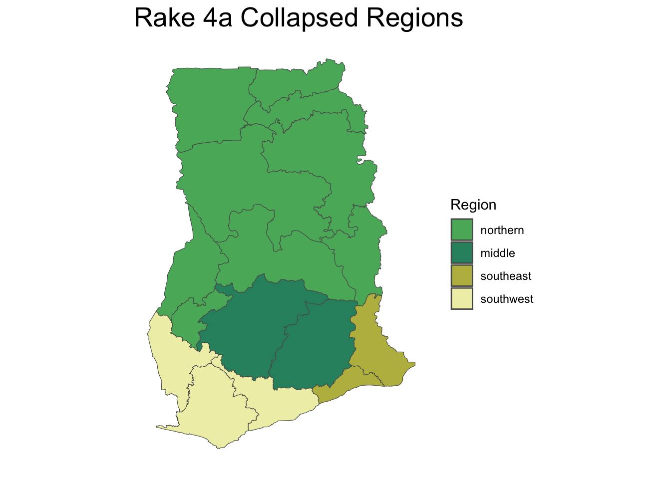
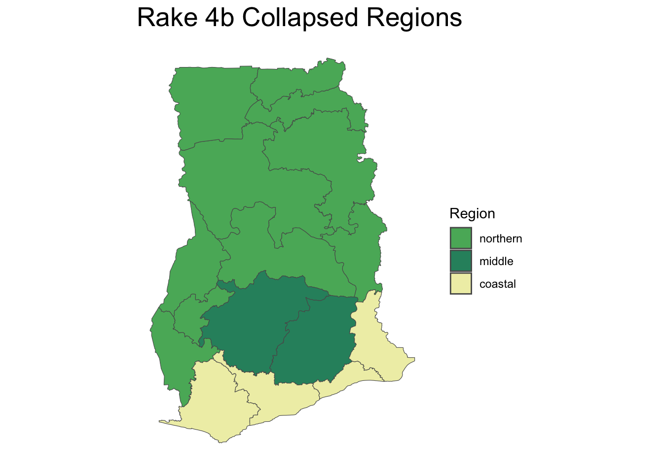
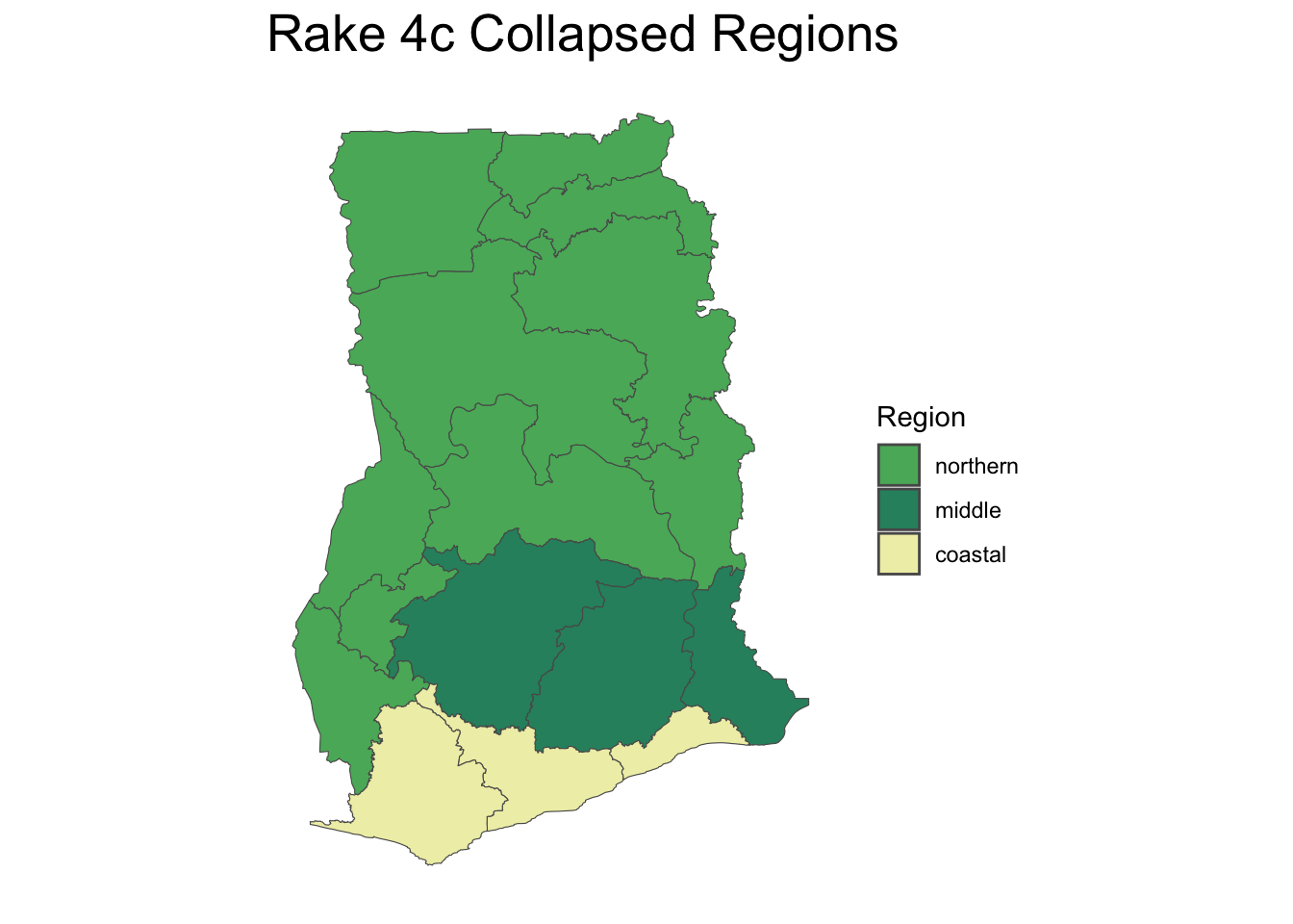
Sensitivity Analysis: Grouping Variations

We explored different regional groupings to ensure robust model performance without convergence issues. Grouping strategies were informed by demographic similarities and household population sizes, ensuring meaningful comparisons and reliable raking results.

Code

ggplot() +
  geom_sf(data = regions, aes(fill = region)) +
  theme_minimal() +
  labs(fill = "Region",
       title = "Regions of Ghana")+
  theme(plot.title = element_text(size = 20)) +
  theme(
    axis.text = element_blank(),  # Remove axis text
    axis.title = element_blank(),  # Remove axis titles
    panel.grid = element_blank()
  )

Code

rake1_regions <- regions %>%
  mutate(collapsed_region = case_when(
  region %in% c("Ashanti", "Eastern") ~ "middle",
  region %in% c("Upper East", "Upper West", "Northern East", "Northern", "Savannah", "Oti", "Bono", "Bono East", "Ahafo") ~ "northern",
  region %in% c("Greater Accra", "Volta") ~ "southeast",
  region %in% c("Central", "Western", "Western North") ~ "southwest",
  TRUE ~ region)) %>%
  mutate(collapsed_region = factor(collapsed_region, levels = c("northern", "middle", "southeast", "southwest")))

# Define custom colors for each region
custom_colors <- c("middle" = "#2b8f6d", 
                   "northern" = "#58b368", 
                   "southeast" = "#bcba50", 
                   "southwest" = "#EFEEB4"
                   )

ggplot() +
  geom_sf(data = rake1_regions, aes(fill = collapsed_region)) +
  scale_fill_manual(values = custom_colors) +
  theme_minimal() +
  labs(fill = "Region",
       title = "Rake 4a Collapsed Regions") +
  theme(plot.title = element_text(size = 20)) +
  theme(
    axis.text = element_blank(),  # Remove axis text
    axis.title = element_blank(),  # Remove axis titles
    panel.grid = element_blank()
  )

Code

rake2_regions <- regions %>%
  mutate(collapsed_region = case_when(
  region %in% c("Ashanti", "Eastern") ~ "middle",
  region %in% c("Upper East", "Upper West", "Northern East", "Northern", "Savannah", "Oti", "Western North", "Bono", "Bono East", "Ahafo") ~ "northern",
  region %in% c("Greater Accra", "Volta", "Central", "Western") ~ "coastal",
  TRUE ~ region)) %>%
  mutate(collapsed_region = factor(collapsed_region, levels = c("northern", "middle", "coastal")))

# Define custom colors for each region
custom_colors <- c("middle" = "#2b8f6d", 
                   "northern" = "#58b368", 
                   "coastal" = "#EFEEB4"
                   )

ggplot() +
  geom_sf(data = rake2_regions, aes(fill = collapsed_region)) +
  scale_fill_manual(values = custom_colors) +
  theme_minimal() +
  labs(fill = "Region",
       title = "Rake 4b Collapsed Regions") +
  theme(plot.title = element_text(size = 20)) +
  theme(
    axis.text = element_blank(),  # Remove axis text
    axis.title = element_blank(),  # Remove axis titles
    panel.grid = element_blank()
  )

Code

rake3_regions <- regions %>%
  mutate(collapsed_region = case_when(
  region %in% c("Ashanti", "Eastern", "Volta") ~ "middle",
  region %in% c("Upper East", "Upper West", "Northern East", "Northern", "Savannah", "Oti", "Western North", "Bono", "Bono East", "Ahafo") ~ "northern",
  region %in% c("Greater Accra", "Central", "Western") ~ "coastal",
  TRUE ~ region)) %>%
  mutate(collapsed_region = factor(collapsed_region, levels = c("northern", "middle", "coastal")))

# Define custom colors for each region
custom_colors <- c("middle" = "#2b8f6d", 
                   "northern" = "#58b368", 
                   "coastal" = "#EFEEB4"
                   )

ggplot() +
  geom_sf(data = rake3_regions, aes(fill = collapsed_region)) +
  scale_fill_manual(values = custom_colors) +
  theme_minimal() +
  labs(fill = "Region",
       title = "Rake 4c Collapsed Regions") +
  theme(plot.title = element_text(size = 20)) +
  theme(
    axis.text = element_blank(),  # Remove axis text
    axis.title = element_blank(),  # Remove axis titles
    panel.grid = element_blank()
  )

Sensitivity Analysis: Results

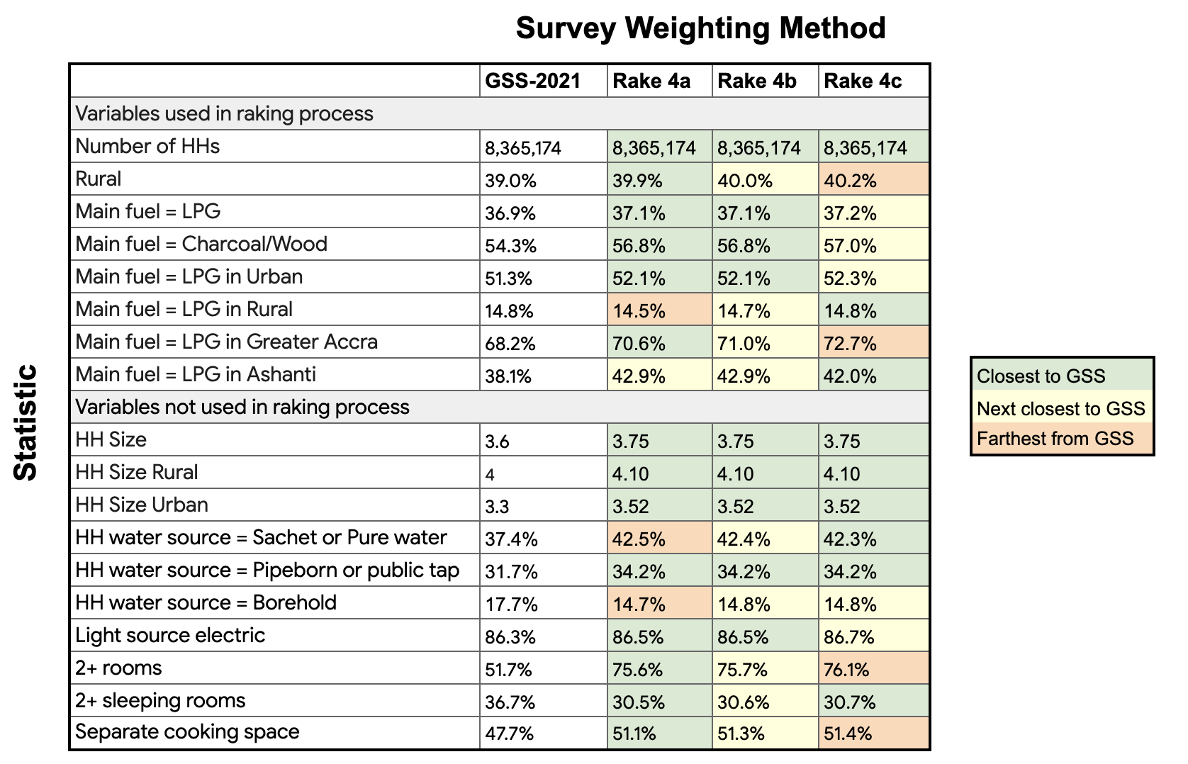
The table below shows the results from our sensitivity analysis and follows a similar format to the previous table. Here, the statistics are broken up by variables used in the raking process and those that were not.

Overall, the results from the sensitivity analysis showed stability across the three groupings. Based on this, the team in Ghana decided which groupings of regions made the most sense based on knowledge of the regions, selecting 4a as their preferred model.

Bibliography:

Battaglia, M., Izrael, D., Hoaglin, D., & Frankel, M. (2004a). Tips and Tricks for Raking Survey Data (aka Sample Balancing). Abt Associates.

Battaglia, M. P., Hoaglin, D. C., & Frankel, M. R. (2009). Practical Considerations in Raking Survey Data. Survey Practice, 2(5). https://doi.org/10.29115/SP-2009-0019

Brick, J. M., Montaquila, J., Roth, S., & Brick, J. M. (2003). IDENTIFYING PROBLEMS WITH RAKING ESTIMATORS.

Calibrating Survey Data using Iterative Proportional Fitting (Raking). (n.d.). https://doi.org/10.1177/1536867X1401400104

DeBell, M., & Krosnick, J. A. (n.d.). Computing Weights for American National Election Study Survey Data.

Kennedy, A. M., Arnold Lau and Courtney. (2018, January 26). 1. How different weighting methods work. Pew Research Center. https://www.pewresearch.org/methods/2018/01/26/how-different-weighting-methods-work/

Citation

BibTeX citation:

@online{white2024,
  author = {White, Lewis},
  title = {Raking to {Improve} {Survey} {Weights}},
  date = {2024-05-03},
  url = {https://lewis-r-white.github.io/posts/2024-05-03-survey-raking/},
  langid = {en}
}

For attribution, please cite this work as:

White, Lewis. 2024. “Raking to Improve Survey Weights.” May 3, 2024. https://lewis-r-white.github.io/posts/2024-05-03-survey-raking/.

Introduction: The Need for Survey Weights

An Overview of the Raking Methodology for Survey Weights

Simple Raking Example

Raking steps:

Simple Raking Example

Case Study: Raking to Improve Representativeness in National Household Survey

Background:

Set Up:

Setting up the Population Totals for Raking

Specifying the Survey Design (using Rake()) for Each of the Models

Calculating the Survey Statistics for Each Model

Results

Conclusions

Sensitivity Analysis: Grouping Variations

Sensitivity Analysis: Results

Bibliography:

Citation

Specifying the Survey Design (using `Rake()`) for Each of the Models